Training a Model

In the last notebook, we learned how to write stock indicators in PyBroker. Indicators are a good starting point for developing a trading strategy. But to create a successful strategy, it is likely that a more sophisticated approach using predictive modeling will be needed.

Fortunately, one of the main features of PyBroker is the ability to train and backtest machine learning models. These models can utilize indicators as features to make more accurate predictions about market movements. Once trained, these models can be backtested using a popular technique known as Walkforward Analysis, which simulates how a strategy would perform during actual trading.

We’ll explain Walkforward Analysis more in depth later in this notebook. But first, let’s get started with some needed imports!

import numpy as np
import pandas as pd
import pybroker
from numba import njit
from pybroker import Strategy, StrategyConfig, YFinance

As with DataSource and Indicator data, PyBroker can also cache trained models to disk. You can enable caching for all three by calling pybroker.enable_caches:

pybroker.enable_caches('walkforward_strategy')

In the last notebook, we implemented an indicator that calculates the close-minus-moving-average (CMMA) using NumPy and Numba. Here’s the code for the CMMA indicator again:

def cmma(bar_data, lookback):

    @njit  # Enable Numba JIT.
    def vec_cmma(values):
        # Initialize the result array.
        n = len(values)
        out = np.array([np.nan for _ in range(n)])

        # For all bars starting at lookback:
        for i in range(lookback, n):
            # Calculate the moving average for the lookback.
            ma = 0
            for j in range(i - lookback, i):
                ma += values[j]
            ma /= lookback
            # Subtract the moving average from value.
            out[i] = values[i] - ma
        return out

    # Calculate for close prices.
    return vec_cmma(bar_data.close)

cmma_20 = pybroker.indicator('cmma_20', cmma, lookback=20)

Train and Backtest

Next, we want to build a model that predicts the next day’s return using the 20-day CMMA. Using simple linear regression is a good approach to begin experimenting with. Below we import a LinearRegression model from scikit-learn:

from sklearn.linear_model import LinearRegression
from sklearn.metrics import r2_score

We create a train_slr function to train the LinearRegression model:

def train_slr(symbol, train_data, test_data):
    # Train
    # Previous day close prices.
    train_prev_close = train_data['close'].shift(1)
    # Calculate daily returns.
    train_daily_returns = (train_data['close'] - train_prev_close) / train_prev_close
    # Predict next day's return.
    train_data['pred'] = train_daily_returns.shift(-1)
    train_data = train_data.dropna()
    # Train the LinearRegession model to predict the next day's return
    # given the 20-day CMMA.
    X_train = train_data[['cmma_20']]
    y_train = train_data[['pred']]
    model = LinearRegression()
    model.fit(X_train, y_train)

    # Test
    test_prev_close = test_data['close'].shift(1)
    test_daily_returns = (test_data['close'] - test_prev_close) / test_prev_close
    test_data['pred'] = test_daily_returns.shift(-1)
    test_data = test_data.dropna()
    X_test = test_data[['cmma_20']]
    y_test = test_data[['pred']]
    # Make predictions from test data.
    y_pred = model.predict(X_test)
    # Print goodness of fit.
    r2 = r2_score(y_test, np.squeeze(y_pred))
    print(symbol, f'R^2={r2}')

    # Return the trained model and columns to use as input data.
    return model, ['cmma_20']

The train_slr function uses the 20-day CMMA as the input feature, or predictor, for the LinearRegression model. The function then fits the LinearRegression model to the training data for that stock symbol.

After fitting the model, the function uses the testing data to evaluate the model’s accuracy, specifically by computing the R-squared score. The R-squared score provides a measure of how well the LinearRegression model fits the testing data.

The final output of the train_slr function is the trained LinearRegression model specifically for that stock symbol, along with the cmma_20 column, which is to be used as input data when making predictions. PyBroker will use this model to predict the next day’s return of the stock during the backtest. The train_slr function will be called for each stock symbol, and the trained models will be used to predict the next day’s return for each individual stock.

Once the function to train the model has been defined, it needs to be registered with PyBroker. This is done by creating a new ModelSource instance using the pybroker.model function. The arguments to this function are the name of the model ('slr' in this case), the function that will train the model (train_slr), and a list of indicators to use as inputs for the model (in this case, cmma_20).

model_slr = pybroker.model('slr', train_slr, indicators=[cmma_20])

To create a trading strategy that uses the trained model, a new Strategy object is created using the YFinance data source, and specifying the start and end dates for the backtest period.

config = StrategyConfig(bootstrap_sample_size=100)
strategy = Strategy(YFinance(), '3/1/2017', '3/1/2022', config)
strategy.add_execution(None, ['NVDA', 'AMD'], models=model_slr)

The add_execution method is then called on the Strategy object to specify the details of the trading execution. In this case, a None value is passed as the first argument, which means that no trading function will be used during the backtest.

The last step is to run the backtest by calling the backtest method on the Strategy object, with a train_size of 0.5 to specify that the model should be trained on the first half of the backtest data, and tested on the second half.

strategy.backtest(train_size=0.5)

Backtesting: 2017-03-01 00:00:00 to 2022-03-01 00:00:00

Loading bar data...
[*********************100%***********************]  2 of 2 completed
Loaded bar data: 0:00:00

Computing indicators...

100% (2 of 2) |##########################| Elapsed Time: 0:00:01 Time:  0:00:01

Train split: 2017-03-01 00:00:00 to 2019-08-28 00:00:00
AMD R^2=-0.006808549721842416
NVDA R^2=-0.004416132743176426
Finished training models: 0:00:00

Finished backtest: 0:00:01

Walkforward Analysis

PyBroker employs a powerful algorithm known as Walkforward Analysis to perform backtesting. The algorithm partitions the backtest data into a fixed number of time windows, each containing a train-test split of data.

The Walkforward Analysis algorithm then proceeds to “walk forward” in time, in the same manner that a trading strategy would be executed in the real world. The model is first trained on the earliest window and then evaluated on the test data in that window.

As the algorithm moves forward to evaluate the next window in time, the test data from the previous window is added to the training data. This process continues until all of the time windows are evaluated.

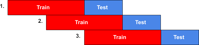
By using this approach, the Walkforward Analysis algorithm is able to simulate the real-world performance of a trading strategy, and produce more reliable and accurate backtesting results.

Let’s consider a trading strategy that generates buy and sell signals from the LinearRegression model that we trained earlier. The strategy is implemented as the hold_long function:

def hold_long(ctx):
    if not ctx.long_pos():
        # Buy if the next bar is predicted to have a positive return:
        if ctx.preds('slr')[-1] > 0:
            ctx.buy_shares = 100
    else:
        # Sell if the next bar is predicted to have a negative return:
        if ctx.preds('slr')[-1] < 0:
            ctx.sell_shares = 100

strategy.clear_executions()
strategy.add_execution(hold_long, ['NVDA', 'AMD'], models=model_slr)

The hold_long function opens a long position when the model predicts a positive return for the next bar, and then closes the position when the model predicts a negative return.

The ctx.preds(‘slr’) method is used to access the predictions made by the 'slr' model for the current stock symbol being executed in the function (NVDA or AMD). The predictions are stored in a NumPy array, and the most recent prediction for the current stock symbol is accessed using ctx.preds('slr')[-1], which is the model’s prediction of the next bar’s return.

Now that we have defined a trading strategy and registered the 'slr' model, we can run the backtest using the Walkforward Analysis algorithm.

The backtest is run by calling the walkforward method on the Strategy object, with the desired number of time windows and train/test split ratio. In this case, we will use 3 time windows, each with a 50/50 train-test split.

Additionally, since our 'slr' model makes a prediction for one bar in the future, we need to specify the lookahead parameter as 1. This is necessary to ensure that training data does not leak into the test boundary. The lookahead parameter should always be set to the number of bars in the future being predicted.

result = strategy.walkforward(
    warmup=20,
    windows=3,
    train_size=0.5,
    lookahead=1,
    calc_bootstrap=True
)

Backtesting: 2017-03-01 00:00:00 to 2022-03-01 00:00:00

Loaded cached bar data.

Loaded cached indicator data.

Train split: 2017-03-06 00:00:00 to 2018-06-01 00:00:00
AMD R^2=-0.007950114729117885
NVDA R^2=-0.04203364470839133
Finished training models: 0:00:00

Test split: 2018-06-04 00:00:00 to 2019-08-30 00:00:00

100% (314 of 314) |######################| Elapsed Time: 0:00:00 Time:  0:00:00

Train split: 2018-06-04 00:00:00 to 2019-08-30 00:00:00
AMD R^2=0.0006422677593683757
NVDA R^2=-0.023591728578221893
Finished training models: 0:00:00

Test split: 2019-09-03 00:00:00 to 2020-11-27 00:00:00

100% (314 of 314) |######################| Elapsed Time: 0:00:00 Time:  0:00:00

Train split: 2019-09-03 00:00:00 to 2020-11-27 00:00:00
AMD R^2=-0.015508227883924253
NVDA R^2=-0.4567200095787838
Finished training models: 0:00:00

Test split: 2020-11-30 00:00:00 to 2022-02-28 00:00:00

100% (314 of 314) |######################| Elapsed Time: 0:00:00 Time:  0:00:00

Calculating bootstrap metrics: sample_size=100, samples=10000...
Calculated bootstrap metrics: 0:00:03

Finished backtest: 0:00:04

During the backtesting process using the Walkforward Analysis algorithm, the 'slr' model is trained on a given window’s training data, and then the hold_long function runs on the same window’s test data.

The model is trained on the training data to make predictions about the next day’s returns. The hold_long function then uses these predictions to make buy or sell decisions for the current day’s trading session.

By evaluating the performance of the trading strategy on the test data for each window, we can see how well the strategy is likely to perform in real-world trading conditions. This process is repeated for each time window in the backtest, using the results to evaluate the overall performance of the trading strategy:

result.metrics_df

	name	value
0	trade_count	43.000000
1	initial_market_value	100000.000000
2	end_market_value	109831.000000
3	total_pnl	12645.000000
4	unrealized_pnl	-2814.000000
5	total_return_pct	12.645000
6	total_profit	20566.000000
7	total_loss	-7921.000000
8	total_fees	0.000000
9	max_drawdown	-14177.000000
10	max_drawdown_pct	-12.272121
11	win_rate	76.744186
12	loss_rate	23.255814
13	winning_trades	33.000000
14	losing_trades	10.000000
15	avg_pnl	294.069767
16	avg_return_pct	5.267674
17	avg_trade_bars	25.488372
18	avg_profit	623.212121
19	avg_profit_pct	9.237576
20	avg_winning_trade_bars	19.151515
21	avg_loss	-792.100000
22	avg_loss_pct	-7.833000
23	avg_losing_trade_bars	46.400000
24	largest_win	2715.000000
25	largest_win_pct	9.320000
26	largest_win_bars	2.000000
27	largest_loss	-5054.000000
28	largest_loss_pct	-16.140000
29	largest_loss_bars	43.000000
30	max_wins	13.000000
31	max_losses	2.000000
32	sharpe	0.023425
33	profit_factor	1.094471
34	ulcer_index	1.177116
35	upi	0.009193
36	equity_r2	0.772082
37	std_error	4191.846954

result.bootstrap.conf_intervals

		lower	upper
name	conf
Profit Factor	97.5%	0.259819	1.296660
	95%	0.303435	1.151299
	90%	0.373167	1.002514
Sharpe Ratio	97.5%	-0.359565	0.050383
	95%	-0.332180	0.018154
	90%	-0.276757	-0.018004

result.bootstrap.drawdown_conf

	amount	percent
conf
99.9%	-13917.50	-12.190522
99%	-11058.25	-9.693729
95%	-8380.25	-7.480589
90%	-7129.00	-6.403027

In summary, we have now completed the process of training and backtesting a linear regression model using PyBroker, with the help of Walkforward Analysis. The metrics that we have seen are based on the test data from all of the time windows in the backtest. Although our trading strategy needs to be improved, we have gained a good understanding of how to train and evaluate a model in PyBroker.

Please keep in mind that before conducting regression analysis, it is important to verify certain assumptions such as homoscedasticity, normality of residuals, etc. I have not provided the details for these assumptions here for the sake of brevity and recommend that you perform this exercise on your own.

We are also not limited to just building linear regression models in PyBroker. We can train other model types such as gradient boosted machines, neural networks, or any other architecture that we choose. This flexibility allows us to explore and experiment with various models and approaches to find the best performing model for our specific trading goals.

PyBroker also offers customization options, such as the ability to specify an input_data_fn for our model in case we need to customize how its input data is built. This would be required when constructing input for autoregressive models (i.e. ARMA or RNN) that use multiple past values to make predictions. Similarly, we can specify our own predict_fn to customize how predictions are made (by default, the model’s predict function is called).

With this knowledge, you can start building and testing your own models and trading strategies in PyBroker, and begin exploring the vast possibilities that this framework offers!